Introduction
In computer science, a Fibonacci heap is a data structure for priority queue operations, consisting of a collection of heap-ordered trees. It has a better amortized running time than many other priority queue data structures including the binary heap and binomial heap (二项堆). Michael L. Fredman and Robert E. Tarjan developed Fibonacci heaps in 1984 and published them in a scientific journal in 1987. Fibonacci heaps are named after the Fibonacci numbers, which are used in their running time analysis.
| Operation | Insert | Find-min | Delete-min | Decrease-key | Merge |
|---|---|---|---|---|---|
| Complexity |
For the Fibonacci heap,
- the find-minimum operation takes constant (O(1)) amortized time1.
- The insert and decrease key operations also work in constant amortized time.
- Deleting an element (most often used in the special case of deleting the minimum element) works in O(log n) amortized time, where n is the size of the heap.
This means that starting from an empty data structure, any sequence of a insert and decrease key operations and b delete operations would take O(a + b log n) worst case time, where n is the maximum heap size. In a binary or binomial heap, such a sequence of operations would take O((a + b) log n) time. ==A Fibonacci heap is thus better than a binary or binomial heap when b is smaller than a by a non-constant factor==.
It is also possible to merge two Fibonacci heaps in constant amortized time, improving on the logarithmic merge time of a binomial heap, and improving on binary heaps which cannot handle merges efficiently.
Using Fibonacci heaps for priority queues improves the asymptotic running time of important algorithms, such as Dijkstra’s algorithm for computing the shortest path between two nodes in a graph, compared to the same algorithm using other slower priority queue data structures.
Structure
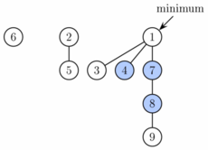
A Fibonacci heap is a collection of trees satisfying the minimum-heap property, that is, the key of a child is always greater than or equal to the key of the parent. This implies that the minimum key is always at the root of one of the trees. Compared with binomial heaps, the structure of a Fibonacci heap is more flexible. The trees do not have a prescribed shape and in the extreme case the heap can have every element in a separate tree. This flexibility allows some operations to be executed in a lazy manner, postponing the work for later operations. For example, merging heaps is done simply by concatenating the two lists of trees, and operation decrease key sometimes cuts a node from its parent and forms a new tree.
斐波那契堆是一种最小堆。与二项堆相比,它更加灵活:没有规定的形状,极端情况下可以每个节点独立成根。这种灵活性允许一些操作采用懒标记的形式,推迟执行时间。 例如,合并堆可以仅连接起两个树的列表,删除关键码的操作可以从其父节点中剪切一个节点并形成一个新的树。
However, at some point order needs to be introduced to the heap to achieve the desired running time. In particular, degrees of nodes (here degree means the number of direct children) are kept quite low: every node has degree at most log n and the size of a subtree rooted in a node of degree k is at least , where is the Fibonacci number. This is achieved by the rule that we can cut at most one child of each non-root node. When a second child is cut, the node itself needs to be cut from its parent and becomes the root of a new tree (see Proof of degree bounds, below). The number of trees is decreased in the operation delete minimum, where trees are linked together.
斐波那契堆也有其特别的要求:尤其是其节点的度(直接孩子的数量)保持非常低——每个节点的度最大不超过 log n,以 k 度节点为根的子树的规模不超过 。 这个规则通过“最多可以切割每个非根节点的一个子节点”的要求来实现。当第二个节点要被删除,则需要从其父节点上切割并成为一个新的子树的根。 树的数量通过 delete minimum 操作来减少——树本身是与其它树互连的。
As a result of a relaxed structure, some operations can take a long time while others are done very quickly. For the amortized running time analysis, we use the potential method, in that we pretend that very fast operations take a little bit longer than they actually do. This additional time is then later combined and subtracted from the actual running time of slow operations. The amount of time saved for later use is measured at any given moment by a potential function. The potential of a Fibonacci heap is given by where t is the number of trees in the Fibonacci heap, and m is the number of marked nodes. A node is marked if at least one of its children was cut since this node was made a child of another node (all roots are unmarked). The amortized time for an operation is given by the sum of the actual time and c times the difference in potential, where c is a constant (chosen to match the constant factors in the O notation for the actual time).
作为一种松散的结构,一些操作花费的时间可能很长,而其他操作则非常快。使用势能分析法来进行分摊计算,留待后续使用而节省的时间量通过势能函数来测量。势能函数是 ,t 是斐波那契堆中的树的数量,m 是被懒惰标记的节点数。 一个节点被标记,仅当至少一个其子节点被剪切,因为该节点是另一个节点的子节点(所有根节点都不会标记) 对一个操作的分摊时间由实际操作时间和 c 倍势能差之和给出,其中 c 是一个常数(通常与 O (实际操作时间)中的常数因子相匹配)
Thus, the root of each tree in a heap has one unit of time stored. This unit of time can be used later to link this tree with another tree at amortized time 0. Also, each marked node has two units of time stored. One can be used to cut the node from its parent. If this happens, the node becomes a root and the second unit of time will remain stored in it as in any other root.
因此,堆中每个树的根节点都存储了一个时间单位,这个时间单位可用于后续连接其它树,因此分摊时间为 0. 而每个标记节点有两份时间单位存储:一份可用于从其父节点剪切,这时它就成为新的树的根,原来的第二份时间单位作为根的时间单位保留下来。
Implementation of operations
To allow fast deletion and concatenation, the roots of all trees are linked using a circular doubly linked list. The children of each node are also linked using such a list. For each node, we maintain its number of children and whether the node is marked. Moreover, we maintain a pointer to the root containing the minimum key.
Operation find minimum is now trivial because we keep the pointer to the node containing it. It does not change the potential of the heap, therefore both actual and amortized cost are constant.
As mentioned above, merge is implemented simply by concatenating the lists of tree roots of the two heaps. This can be done in constant time and the potential does not change, leading again to constant amortized time.
Operation insert works by creating a new heap with one element and doing merge. This takes constant time, and the potential increases by one, because the number of trees increases. The amortized cost is thus still constant.
Operation extract minimum (same as delete minimum) operates in three phases. First we take the root containing the minimum element and remove it. Its children will become roots of new trees. If the number of children was d, it takes time O(d) to process all new roots and the potential increases by d−1. Therefore, the amortized running time of this phase is O(d) = O(log n).
However to complete the extract minimum operation, we need to update the pointer to the root with minimum key. Unfortunately there may be up to n roots we need to check. In the second phase we therefore decrease the number of roots by successively linking together roots of the same degree. When two roots u and v have the same degree, we make one of them a child of the other so that the one with the smaller key remains the root. Its degree will increase by one. This is repeated until every root has a different degree. To find trees of the same degree efficiently we use an array of length O(log n) in which we keep a pointer to one root of each degree. When a second root is found of the same degree, the two are linked and the array is updated. The actual running time is O(log n + m) where m is the number of roots at the beginning of the second phase. At the end we will have at most O(log n) roots (because each has a different degree). Therefore, the difference in the potential function from before this phase to after it is: O(log n) − m, and the amortized running time is then at most O(log n + m) + c(O(log n) − m). With a sufficiently large choice of c, this simplifies to O(log n).
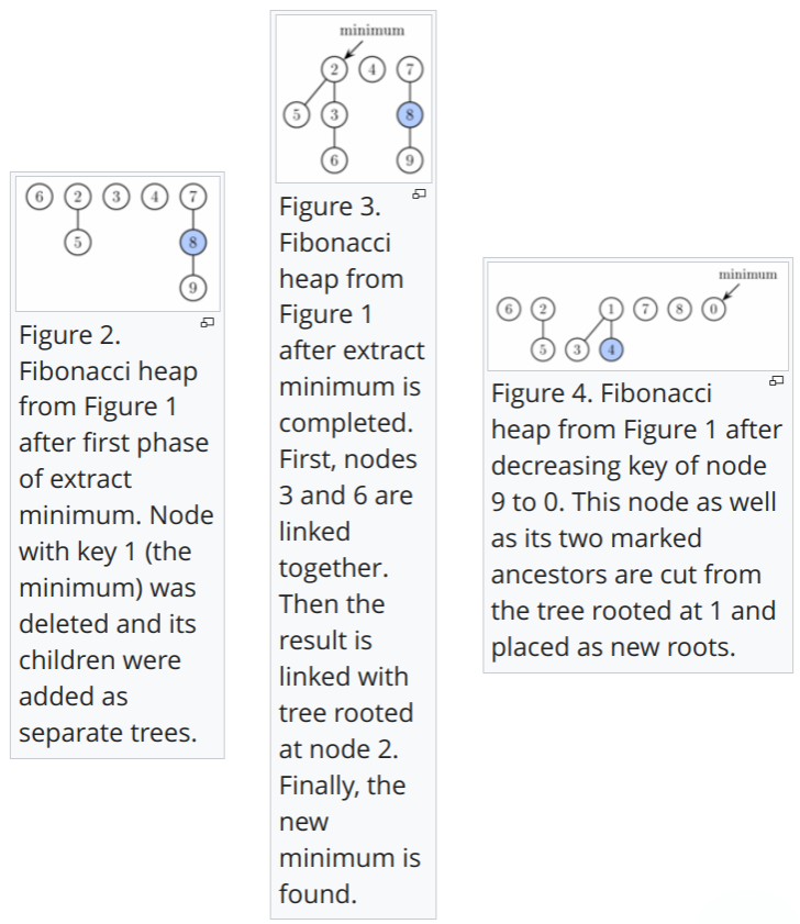
In the third phase we check each of the remaining roots and find the minimum. This takes O(log n) time and the potential does not change. The overall amortized running time of extract minimum is therefore O(log n).
Operation decrease key will take the node, decrease the key and if the heap property becomes violated (the new key is smaller than the key of the parent), the node is cut from its parent. If the parent is not a root, it is marked. If it has been marked already, it is cut as well and its parent is marked. We continue upwards until we reach either the root or an unmarked node. Now we set the minimum pointer to the decreased value if it is the new minimum. In the process we create some number, say k, of new trees. Each of these new trees except possibly the first one was marked originally but as a root it will become unmarked. One node can become marked. Therefore, the number of marked nodes changes by −(k − 1) + 1 = − k + 2. Combining these 2 changes, the potential changes by 2 (−k + 2) + k = −k + 4. The actual time to perform the cutting was O(k), therefore (again with a sufficiently large choice of c) the amortized running time is constant.
Finally, operation delete can be implemented simply by decreasing the key of the element to be deleted to minus infinity, thus turning it into the minimum of the whole heap. Then we call extract minimum to remove it. The amortized running time of this operation is O(log n).
Proof of degree bounds
The amortized performance of a Fibonacci heap depends on the degree (number of children) of any tree root being O(log n), where n is the size of the heap. Here we show that the size of the (sub) tree rooted at any node x of degree d in the heap must have size at least Fd+2, where Fk is the _k_th Fibonacci number. The degree bound follows from this and the fact (easily proved by induction) that 


Consider any node x somewhere in the heap (x need not be the root of one of the main trees). Define size(x) to be the size of the tree rooted at x (the number of descendants of x, including x itself). We prove by induction on the height of x (the length of a longest simple path from x to a descendant leaf), that size(x) ≥ Fd+2, where d is the degree of x.
Base case: If x has height 0, then d = 0, and size(x) = 1 = _F_2.
Inductive case: Suppose x has positive height and degree d > 0. Let _y_1, _y_2, …, yd be the children of x, indexed in order of the times they were most recently made children of x (_y_1 being the earliest and yd the latest), and let _c_1, _c_2, …, cd be their respective degrees. We claim that ci ≥ i-2 for each i with 2 ≤ i ≤ d: Just before yi was made a child of x, _y_1,…,yi−1 were already children of x, and so x had degree at least i−1 at that time. Since trees are combined only when the degrees of their roots are equal, it must have been that yi also had degree at least i-1 at the time it became a child of x. From that time to the present, yi can only have lost at most one child (as guaranteed by the marking process), and so its current degree ci is at least i−2. This proves the claim.
Since the heights of all the yi are strictly less than that of x, we can apply the inductive hypothesis to them to get size(yi) ≥ Fci+2 ≥ F(i−2)+2 = Fi. The nodes x and _y_1 each contribute at least 1 to size(x), and so we have

A routine induction proves that 
Worst case
Although Fibonacci heaps look very efficient, they have the following two drawbacks:
- They are complicated to implement.
- They are not as efficient in practice when compared with theoretically less efficient forms of heaps. In their simplest version they require storage and manipulation of four pointers per node, whereas only two or three pointers per node are needed in other structures, such as the binary heap, binomial heap, pairing heap, Brodal queue and rank-pairing heap.
Although the total running time of a sequence of operations starting with an empty structure is bounded by the bounds given above, some (very few) operations in the sequence can take very long to complete (in particular delete and delete minimum have linear running time in the worst case). For this reason Fibonacci heaps and other amortized data structures may not be appropriate for real-time systems. It is possible to create a data structure which has the same worst-case performance as the Fibonacci heap has amortized performance. One such structure, the Brodal queue, is, in the words of the creator, “quite complicated” and “[not] applicable in practice.” Created in 2012, the strict Fibonacci heap is a simpler (compared to Brodal’s) structure with the same worst-case bounds. Despite having simpler structure, experiments show that in practice the strict Fibonacci heap performs slower than more complicated Brodal queue and also slower than basic Fibonacci heap. The run-relaxed heaps of Driscoll et al. give good worst-case performance for all Fibonacci heap operations except merge.
Summary of running times
Here are time complexities of various heap data structures. Function names assume a min-heap. For the meaning of “O(f)” and “Θ(f)” see Big O notation.
| Operation | find-min | delete-min | insert | decrease-key | meld |
|---|---|---|---|---|---|
| Binary | Θ(1) | Θ(log n) | O(log n) | O(log n) | Θ(n) |
| Leftist | Θ(1) | Θ(log n) | Θ(log n) | O(log n) | Θ(log n) |
| Binomial | Θ(1) | Θ(log n) | Θ(1) | Θ(log n) | O(log n) |
| Skew binomial | Θ(1) | Θ(log n) | Θ(1) | Θ(log n) | O(log n) |
| Pairing | Θ(1) | O(log n) | Θ(1) | o(log n) | Θ(1) |
| Rank-pairing | Θ(1) | O(log n) | Θ(1) | Θ(1) | Θ(1) |
| Fibonacci | Θ(1) | O(log n) | Θ(1) | Θ(1) | Θ(1) |
| Strict Fibonacci | Θ(1) | O(log n) | Θ(1) | Θ(1) | Θ(1) |
| Brodal | Θ(1) | O(log n) | Θ(1) | Θ(1) | Θ(1) |
| 2–3 heap | O(log n) | O(log n) | O(log n) | Θ(1) | ? |
- Amortized time.
- Brodal and Okasaki describe a technique to reduce the worst-case complexity of meld to Θ(1); this technique applies to any heap datastructure that has insert in Θ(1) and find-min, delete-min, meld in O(log n).
- Lower bound of
upper bound of
- Brodal and Okasaki later describe a persistent variant with the same bounds except for decrease-key, which is not supported. Heaps with n elements can be constructed bottom-up in O(n).

Practical considerations
Fibonacci heaps have a reputation for being slow in practice due to large memory consumption per node and high constant factors on all operations. Recent experimental results suggest that Fibonacci heaps are more efficient in practice than most of its later derivatives, including quake heaps, violation heaps, strict Fibonacci heaps, rank pairing heaps, but less efficient than either pairing heaps or array-based heaps.
External links
- Java applet simulation of a Fibonacci heap
- MATLAB implementation of Fibonacci heap
- De-recursived and memory efficient C implementation of Fibonacci heap (free/libre software, CeCILL-B license)
- Ruby implementation of the Fibonacci heap (with tests)
- Pseudocode of the Fibonacci heap algorithm
- Various Java Implementations for Fibonacci heap
Footnotes
-
Cormen, Thomas H.; Leiserson, Charles E.; Rivest, Ronald L.; Stein, Clifford (2001) [1990]. “Chapter 20: Fibonacci Heaps”. Introduction to Algorithms (2nd ed.). MIT Press and McGraw-Hill. pp. 476–497. ISBN 0-262-03293-7. Third edition p. 518. ↩