90-Priority

应用

应用举例

离散事件模拟
操作系统：任务调度/中断处理/MRU/…
输入法：词频调整

极值元素：须反复地、快速地定位

集合组成：可动态变化
元素优先级：可动态变化

查找极值元素，作为底层数据结构所支持的高效操作，是很多高效算法的基础

内部、外部、在线排序
贪心算法：Huffman编码、Kruskal
平面扫描算法中的事件队列

ADT

template <typename T> struct PQ { //priority queue
	virtual void insert( T ) = 0;
	virtual T getMax() = 0;
	virtual T delMax() = 0;
}; //作为ADT的PQ有多种实现方式，各自的效率及适用场合也不尽相同

Stack 和 Queue，都是 PQ 的特例——优先级完全取决于元素的插入次序
Steap 和 Queap，也是 PQ 的特例——插入和删除的位置受限

实现

Vector

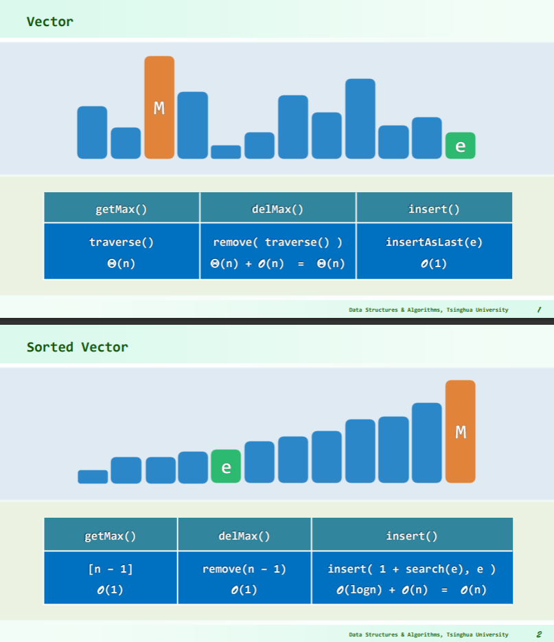
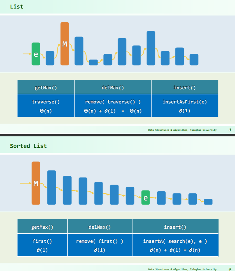
List

BBST

AVL、Splay、Red-black：三个接口均只需 O(logn)时间，但是，BBST 的功能远远超出了 PQ 的需求…
PQ = 1 × insert () + 0.5 × search () + 0.5 × remove ()
若只需查找极值元，则不必维护所有元素之间的全序关系，偏序足矣，因此有理由相信，存在某种更为简单、维护成本更低的实现方式，使得各功能接口的时间复杂度依然为 O (logn)，而且实际效率更高。
当然，就最坏情况而言，这类实现方式已属最优——为什么？

完全二叉堆

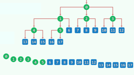
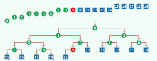完全二叉堆的逻辑元素、物理节点依层次遍历次序彼此对应：

逻辑上等同于完全二叉树
物理上直接使用向量实现
内部节点的最大秩= $⌊ \frac{n - 2}{2} ⌋$ = $⌈ \frac{n - 3}{2} ⌉$
堆序性：只要 0<i，必满足 H[i]<=H[Parent(i)]，即 H[0] 已是全局最大者。

#define Parent(i) ( ((i) - 1) >> 1 )
#define LChild(i) ( 1 + ((i) << 1) )
#define RChild(i) ( (1 + (i)) << 1 )

template <typename T>
struct PQ_ComplHeap : public PQ<T>, public Vector<T> { //完全二叉堆
   PQ_ComplHeap() {} //默认构造
   PQ_ComplHeap( T* A, Rank n ) { copyFrom( A, 0, n ); heapify( _elem, n ); } //批量构造
   void insert( T ); //按照比较器确定的优先级次序，插入词条
   T getMax(); //读取优先级最高的词条
   T delMax(); //删除优先级最高的词条
}; // PQ_ComplHeap
template <typename T> void heapify( T* A, Rank n ); // Floyd建堆算法
template <typename T> Rank percolateDown( T* A, Rank n, Rank i ); //下滤
template <typename T> Rank percolateUp( T* A, Rank i ); //上滤

template <typename T> T PQ_ComplHeap<T>::getMax() { return _elem[0]; }

完全二叉堆的实现

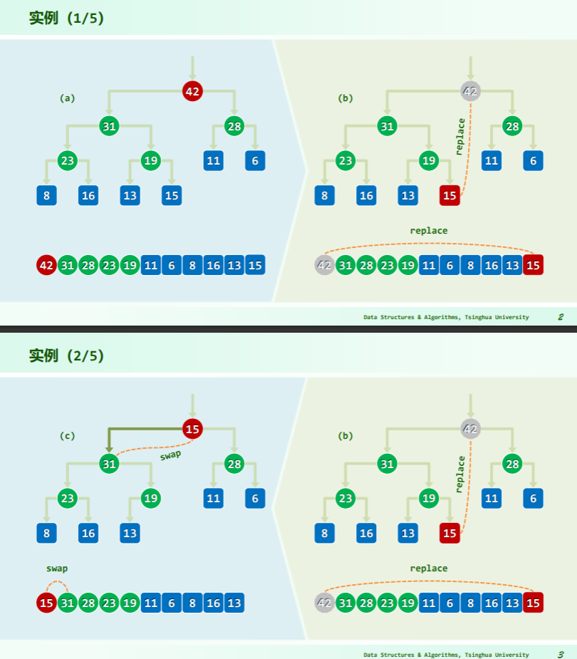
插入

逐层上滤

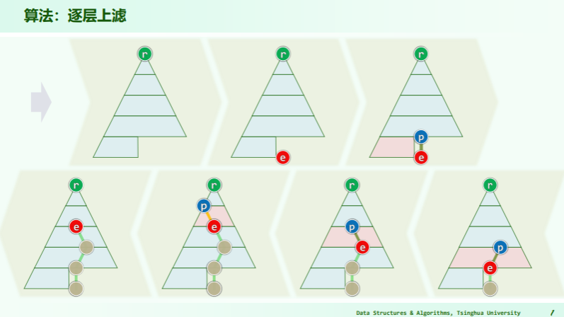
比较位置是： $i = ⌊ \frac{i - 1}{2} ⌋$ ;
父子的秩关系是：父 i，左子 2i+1，右子 2i+2（从 0 开始作秩）；

代码

template <typename T> void PQ_ComplHeap<T>::insert( T e ) { //将词条插入完全二叉堆中
   Vector<T>::insert( e ); //将新词条接至向量末尾
   percolateUp( _elem, _size - 1 ); //再对该词条实施上滤调整
}

template <typename T> Rank percolateUp( T* A, Rank i ) { //对词条A[i]做上滤，0 <= i < _size
   while ( 0 < i ) { //在抵达堆顶之前，反复地
      Rank j = Parent( i ); //考查[i]之父亲[j]
      if ( lt( A[i], A[j] ) ) break; //一旦父子顺序，上滤旋即完成；否则
      swap( A[i], A[j] ); i = j; //父子换位，并继续考查上一层
   } //while
   return i; //返回上滤最终抵达的位置
}

效率

e 在上滤过程中，只可能与祖先们交换
完全树必平衡，e 的祖先不超过 O (logn)个
故知插入操作可在 O (logn)时间内完成
然而就数学期望而言，实际效率往往远远更高（因为不是总要上滤到根）

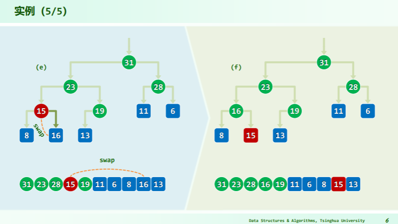
删除

逐层下滤

取尾元素与被删除点——根作替换；
再逐层下滤尾元素直到不小于其后代；

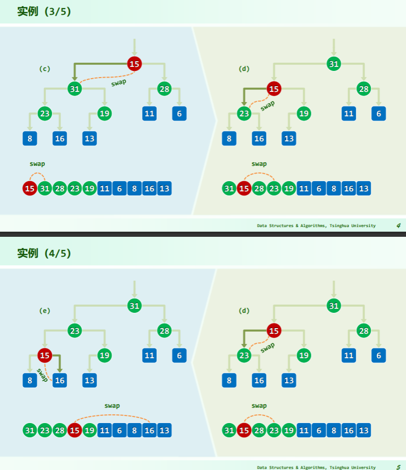
每一次向后比较的秩有如下关系：比较 2i+1 处的元素

代码

#define  ProperParent(PQ, n, i) /*父子（至多）三者中的大者*/ \
            ( RChildValid(n, i) ? Bigger( PQ, Bigger( PQ, i, LChild(i) ), RChild(i) ) : \
            ( LChildValid(n, i) ? Bigger( PQ, i, LChild(i) ) : i \
            ) \
            ) //相等时父节点优先，如此可避免不必要的交换

template <typename T> T PQ_ComplHeap<T>::delMax() { //取出最大词条
   swap( _elem[0], _elem[--_size] ); //堆顶、堆尾互换
   percolateDown( _elem, _size, 0 ); //新堆顶下滤
   return _elem[_size]; //返回原堆顶
}

//对向量前n个词条中的第i个实施下滤，i < n
template <typename T> Rank percolateDown( T* A, Rank n, Rank i ) {
   Rank j; // i及其（至多两个）孩子中，堪为父者
   while ( i != ( j = ProperParent( A, n, i ) ) ) //只要i非j，则
      swap( A[i], A[j] ), i = j; //二者换位，并继续考查下降后的i
   return i; //返回下滤抵达的位置（亦i亦j）
}

如何确保下滤操作正确性？即如何确保交换的节点是最大者？——ProperParent macro 定义了取父子三者中的最大者

效率

e 在每一高度至多交换一次，累计交换不超过 O (logn)次
通过下滤，可在 O (logn)时间内，删除堆顶节点，并整体重新调整为堆
数学期望呢？O (logn) 因为堆底的元素通常较小

建堆

自上而下的上滤

template <typename T> void heapify( T* A, const Rank n ) { //蛮力建堆算法，O(nlogn)时间
   for ( Rank i = 1; i < n; i++ ) //自顶而下，依次
      percolateUp( A, i ); //经上滤插入各节点
}

从第一个节点开始，依次作为堆底，层层上滤；

效率：

最坏情况下，每个节点都需上滤至根（非递减序列），所需成本线性正比于其深度
即便只考虑底层，n/2 个叶节点，深度均为 O (logn) ，亦累计耗时 O (nlogn)
这样长的时间，本足以全排序！所以应该能够更快的

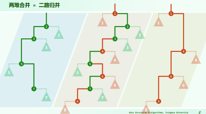
自下而上的下滤

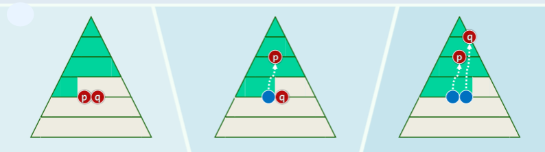
Floyd 建堆法：

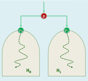
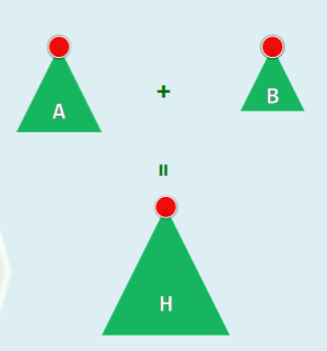
对任意给定的对 H0 和 H1，以及节点p
为得到 $H 0 \cup {p} \cup H 1$ ，只需将堆的根 r0 和 r1 分别作为 p 的左子或右子，再对 p 作下滤即可；

template <typename T> void heapify( T* A, const Rank n ) { //Floyd建堆算法，O(n)时间
   for ( Rank i = n / 2 - 1; - 1 != i; i-- ) //自底而上，依次
      percolateDown( A, n, i ); //经下滤合并子堆
}//可理解为子堆的逐层合并，堆序性最终必然在全局恢复

效率：

每个内部节点所需的调整时间，正比于其高度而非深度
不失一般性，考查满树： $n = 2^{h + 1} - 1$
所有节点的高度总和

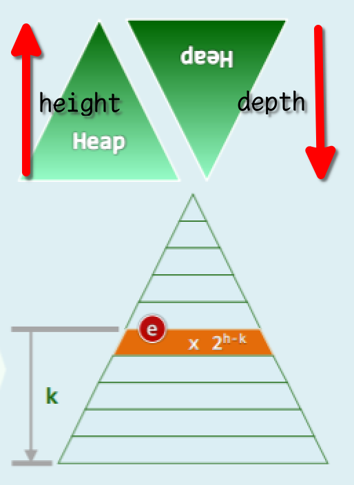
S (n) = k = 1 \sum h k \cdot 2^{h - k} = k = 1 \sum h i = 1 \sum k 2^{h - k} = i = 1 \sum h k = i \sum h 2^{h - k} = i = 1 \sum h k = 0 \sum h - i 2^{k} = i = 1 \sum h (2^{h - i + 1} - 1) = i = 1 \sum h 2^{h - i + 1} - h = i = 1 \sum h 2^{i} - h = 2^{h + 1} - 2 - h = O (n)

[! example] 对 n 个元素进行 Floyd 建堆，最多做多少次数据比较？（不使用 big-O-notation）思路：一个按层序遍历有序满二叉树能达到最多，在按照每层都要下坠底部为止。然后比较次数就是调整次数乘二。上面那个题我的理解是这样：最坏情况里，一个递增序列建成小顶堆，用下滤法从堆底一层层向上调整，可以预见堆顶只需要置换一次，第二层置换两次，依次取决于该层的节点数 2^(k-1)，每次调整都进行兄弟、父子两次比较（不是左右孩子），然后根据等比数列求和计算

思考

Floyd 法在什么场合不适用？——在线建堆时
借助完全堆，可以在 O (nlogn)时间内构造 Huffman 树——小顶堆
大顶堆的 delMin 操作，能否在 O (logn)时间内完成？
- 光凭 max-heap 是无法做到的，delMin 的时间复杂度是 O(n/2)+O (1)+O (logn)=O (n). 分析如下：
- Essentially what you will need to do is search through all the leaf nodes of the implicit heap stored in the array. It will be a leaf node of the heap because its parent must be larger than it (max heap property) and we know the leaves are stored from index n/2 and beyond (though this will not hurt our algorithmic complexity). So essentially what you should do is the following:
  - Search the array for the minimum element
  - Place the last-inserted heap element in the position of the minimum element (essentially this is the delete)
  - Upheap the replaced node to restore maximum heap property and correct storage of the heap in the array
- This will take O (n) for the search of the minimum element, then O (1) for the switch, and finally O (log n) for the upheap. In total this is linear time, essentially the best you can do.
- Remember to be careful with the the index operations, 2*i is the left child of node i and 2*i+1 is the right child of node i in an array based heap (assuming 0th element of the array is always empty and the root of the heap is at index 1)
- 如果建立 min-max heap，则可以在 O (logn)时间内 delMin 和 delMax。

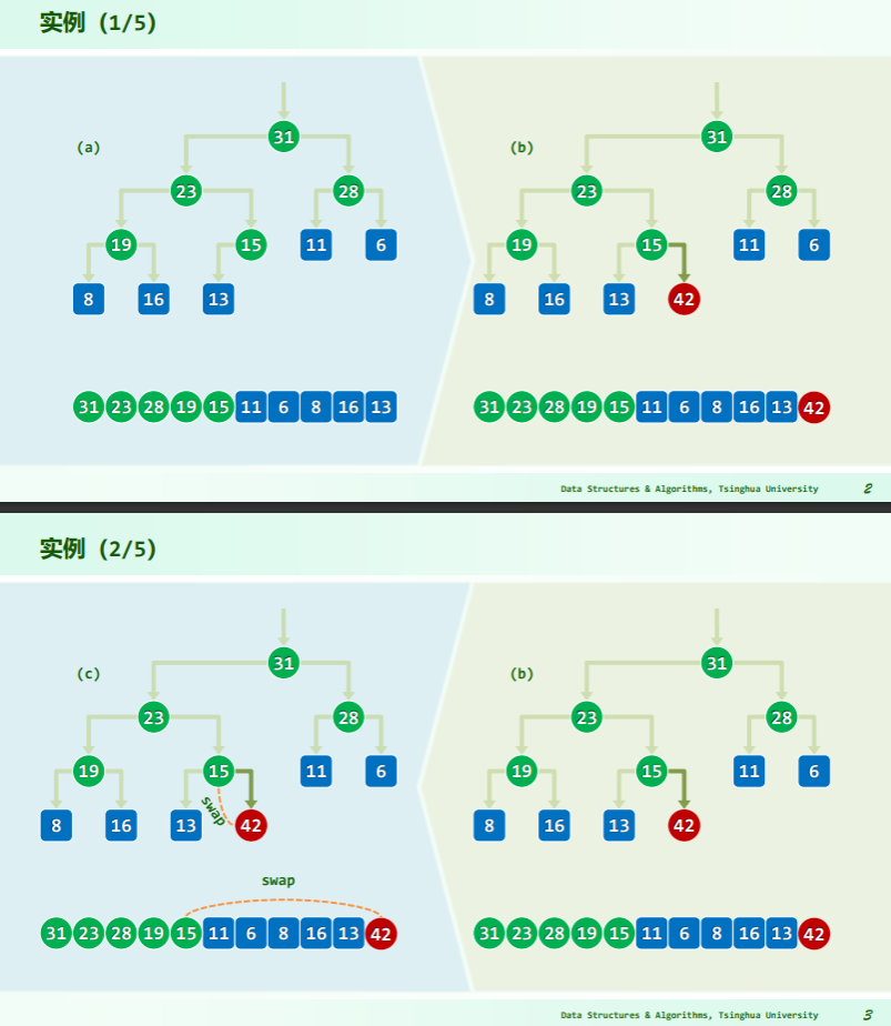
堆排序

思路

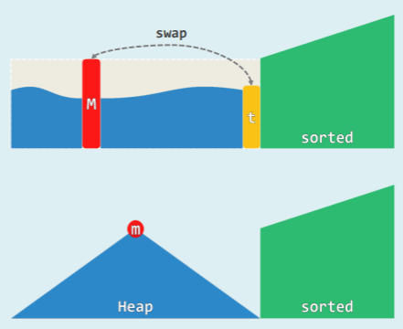
在 selectionSort ()中将 Unsorted 替换为 Heap
初始化： heapify ()，O (n)
迭代： delMax ()，O (logn)
不变性： H ⇐ S
时间复杂度 O(n) + n x O(logn) = O(nlogn)

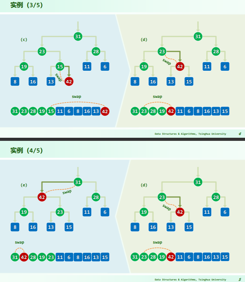
并且由于堆的结构，只需要 swap 就可以实现元素移动：

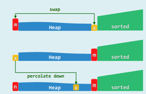
在物理上完全二叉堆即是向量
既然此前有：m = H[ 0 ] , x = H[ n − 1 ]
不妨随即就：swap ( m , x ) = H.insert ( x ) + S.insert ( m )

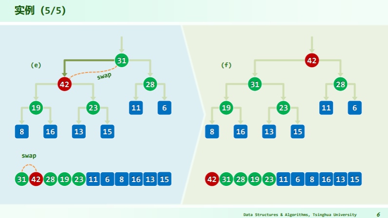
实现

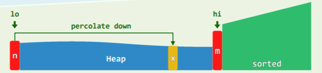
template <typename T> void Vector<T>::heapSort( Rank lo, Rank hi ) { // 0 <= lo < hi <= size，就地堆排序
	T* A = _elem + lo; 
	Rank n = hi - lo; 
	heapify( A, n ); //将待排序区间建成一个完全二叉堆，O(n)
	
	while ( 0 < --n ) {
	//反复地摘除最大元并归入已排序的后缀，直至堆空
		swap( A[0], A[n] );
		percolateDown( A, n, 0 );
	} //堆顶与末元素对换，再下滤
}

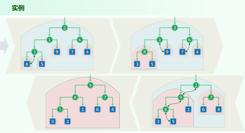
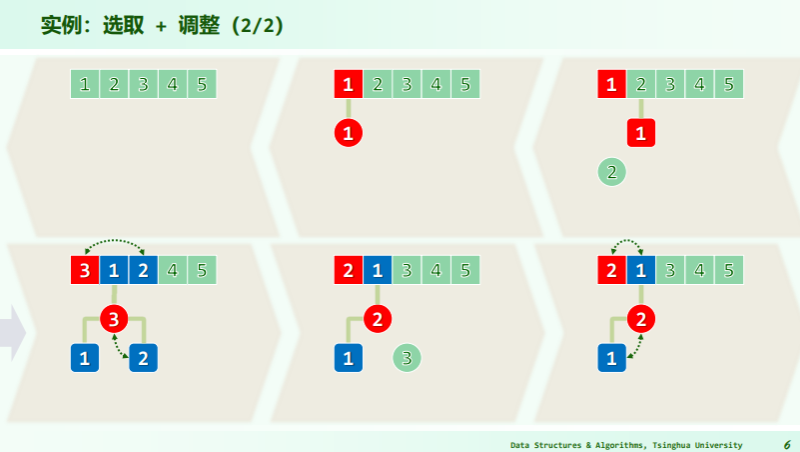
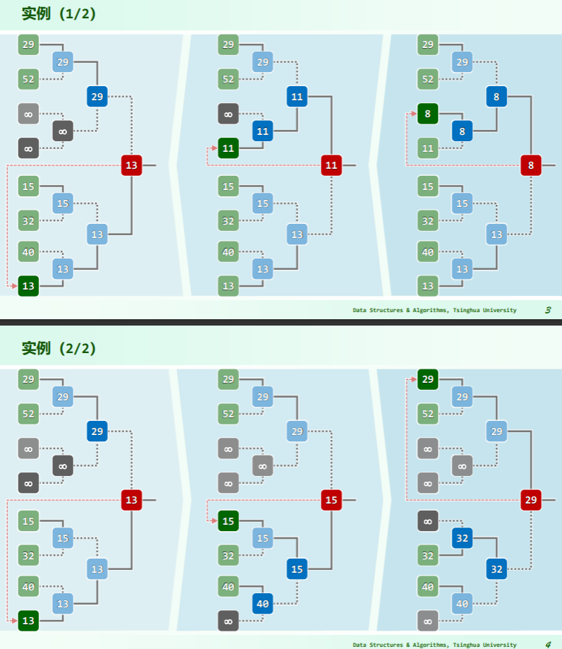
实例

性能

Algorithm	Average	Best	Worst	Auxiliary Space	Stability	Features
HeapSort	O (nlogn)	O (nlogn)	O (nlogn)	O (1)	not stable	规模大时优势明显

使用堆排序，可以在不全排序的情况下找出前 k 个词条，即 O (klogn)的 selection 算法
权衡：就地是否值得——swap 操作涉及两个完整词条，操作的单位成本增加，且不能在线排序。

[! note] Why heapsort unstable? Can it be improved? The heap sort algorithm is not a stable algorithm. This algorithm is not stable because the operations that are performed in a heap can change the relative ordering of the equivalent keys. More detailed: Why Isn’t Heapsort Stable? | Baeldung on Computer Science

How to improve it?

图的合成数解决 Prim 歧义的思想 6-23 合成数法消除 Prim 和 Dijkstra 算法的歧义性。

增加扰动也可以，但只适用于整数作数据域的情况。这些思想的本质还是将重复的关键码改进成单一的关键码。实际上堆排序的不稳定性，是其算法原理的固有不足：10-14 HeapSort 稳定性分析

锦标赛排序

胜者树

一种完全二叉树，其叶节点是参赛选手，内部节点：孩子对决后的胜者，或有重复（连胜）
ADT：
- create () //O (n)
- remove () //O (logn)
- insert () //O (logn)
树根总是全局冠军：类似于堆顶

用以排序的思路

TournamentSort():
	CREATE a tournament tree for the input list
	while there are active leaves
		REMOVE the root
		RETRACE the root down to its leaf
		DEACTIVATE the leaf
		REPLAY along the path back to the root

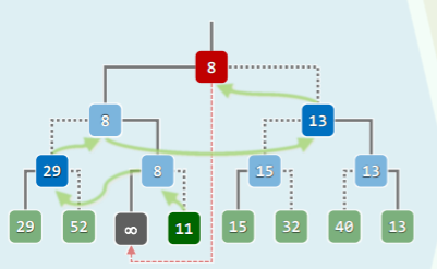
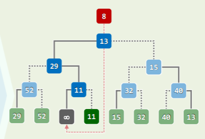
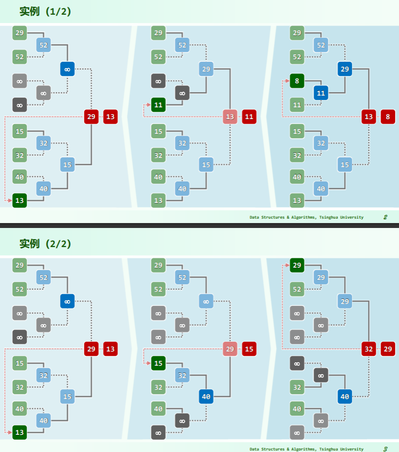
实例

数值小代表胜者；
每一次决出胜者，就将胜者对应的节点设置为无穷大——重赛时不必考虑

性能

空间： O (节点数) = O (叶节点数) = O (n)
构造：仅需 O (n)时间
更新：每次都须全体重赛 replay ？
- 唯上一优胜者的祖先，才有必要！为此，只需从其所在叶节点出发，逐层上溯直到树根，
- 如此，为确定各轮优胜者，总共所需时间仅 O (logn)
时间： n 轮重赛 = n * O (logn) = O (nlogn)，达到下界
稳定性：稳定
用以 k 选取：初始化 O (n)，迭代 k 步 O (klogn)
- 渐进意义上与小顶堆旗鼓相当
- 单就常系数而言，远小于小顶堆——小顶堆在 Floyd 建堆、delMin 的 percolateDown() 中每一层都需要 2 次比较，累计 2*logn 次，胜者树只需要与兄弟比较即可—— logn；

败者树

可以看到，胜者树在重赛过程中，会交替访问沿途节点及其兄弟：

若在内部节点反其道而行之，记录对应比赛的败者，并增设根的“父节点”记录冠军：

注意此时根节点并不是“亚军”

实例

多叉堆

利用优先级队列改进 PFS 框架的思路

回顾图的 PFS 以及统一框架：g→pfs ()：

无论何种算法，差异仅在于所采用的优先级更新器 prioUpdater()
Prim 算法： g→pfs( 0, PrimPU() );
Dijkstra 算法： g→pfs ( 0, DijkPU () );
每一节点引入遍历树后，都需要更新树外顶点的优先级（数），并选出新的优先级最高者
若采用邻接表，两类操作的累计时间分别为 O(n+e) 和 O(n^2) 能否更快呢？——将 PFS 中各顶点组织为优先级队列：
为此需要使用 PQ 接口：
- heapify(): 由 n 个顶点创建初始 PQ 总计 O (n)
- delMax(): 取优先级最高（极短）跨边 (u, w) 总计 O ( n * logn )
- increase(): 更新所有关联顶点到 U 的距离，提高优先级，总计 O ( e * logn )
- 总体运行时间 = O ( (n+e) logn )
- 对于稀疏图，处理效率很高
- 对于稠密图，反而不如常规实现的版本——有无更好的办法？

多叉堆形式

多叉堆 d-heap 仍可基于向量实现，且父、子节点的秩可简明地相互换算
- $p a re n t (k) = ⌊(k - 1) / d ⌋$
- $c hi l d (k, i) = k d + i, 0 < i \leq d$
- d 不是 2 的幂时，不能借助移位加速秩的换算
heapify ()：O (n) //不可能再快了
delMax ()：O (logn) //实质就是 percolateDown ()，已是极限了——为什么？
increase()：O(logn) //实质就是 percolateUp() —— 似乎仍有改进空间…

多叉堆特点

若将二叉堆改成多叉堆，则

堆高降低至 $O (lo g_{d} n)$
相应地，上滤成本降低至 $lo g_{d} n$
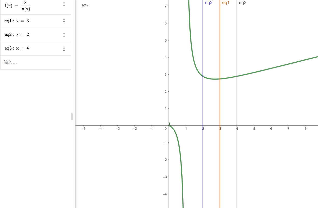
但下滤成本反而增加，只要 d>4，就增加至 $d \cdot lo g_{d} n = \frac{d}{l n d} ln n$
- 可以由函数的极值得知，当 d=e 时，成本最低，而多叉堆 d>=3，因此 d=3 时成本最低，为 $\frac{3}{l n 3} ln n$ ，相较于完全二叉堆
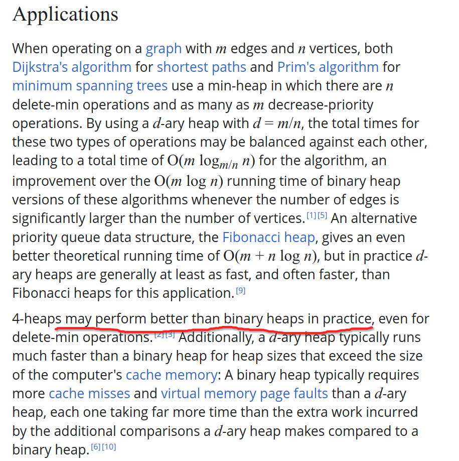
- 并且，根据 wiki 上的描述，4-ary heap 的任何操作效率，都比 binary heap 更高：

更详细的说明

多叉堆实现 PFS 的优势

使用多叉堆实现 PFS 时，运行时间将是 $n \cdot d \cdot lo g_{d} n + e \cdot lo g_{d} n = (n \cdot d + e) lo g_{d} n$
取 $d \approx \frac{e}{n} + 2$ 时总体性能达到最优： $O (e lo g_{\frac{e}{n + 2}} n)$
对于稀疏图仍然能保持高效： $e lo g_{\frac{e}{n + 2}} n \approx n \cdot lo g_{\frac{n}{n + 2}} n = O (n lo g n)$
对于稠密图改进极大： $e lo g_{\frac{e}{n + 2}} n \approx n^{2} \cdot lo g_{\frac{n ^{2}}{n + 2}} n \approx n^{2} = O (e)$

Fibonacci 堆

93-Fibonacci-heap

左式堆

堆合并问题

H = merge (A, B)：将堆 A 和 B 合二为一 //不妨设|A| = n >= m = |B|
方法一：在 A 堆中逐个插入 B 的最大值
- while(!B.empty()) A.insert ( B.delMax ());，直到 B 堆空
- 用时：O(m*(logm + log(n+m))) = O(m*log(n + m))
方法二：直接合并 A 和 B 堆（堆的实现是向量），再 Floyd 建堆
- union( A, B ).heapify( n + m )
- 用时：O(m + n)

有没有更好的办法？比如可否奢望在 O(logn) 时间内实现 merge()？

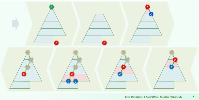
思路

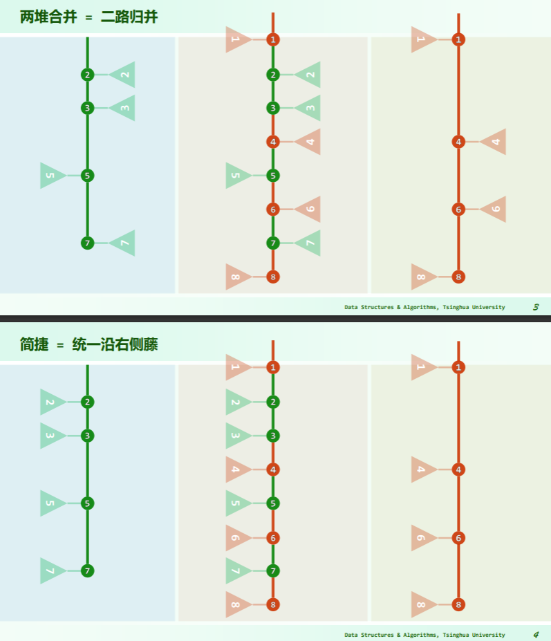
若将“藤”拉直，并统一节点在左、藤在右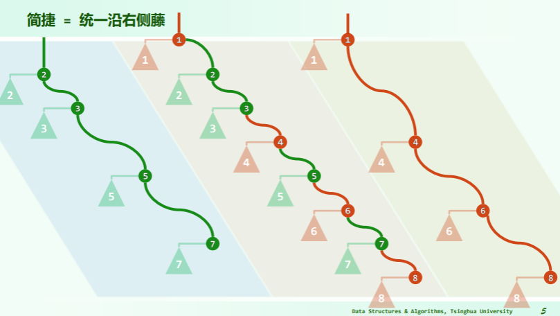：可见，在保证堆序性的前提下附加新的条件，使得在堆的合并过程中，只需调整很少的节点，可以达到高效的合并。

左式堆形态

保持堆序性，附加新条件，使得在堆合并过程中，只涉及少量节点：O (logn)
新条件 = 单侧倾斜：节点分布偏向于左侧，合并操作只涉及右侧
可是，果真如此，则拓扑上不见得是完全二叉树，结构性无法保证！？是的，实际上，结构性并非堆结构的本质要求——堆序性才是堆结构的关键所在。

左式堆的 ADT

template <typename T>
class PQ_LeftHeap : public PQ<T>, public BinTree<T> { //基于二叉树，以左式堆形式实现的PQ
 public:
	PQ_LeftHeap() {} //默认构造
	PQ_LeftHeap( T* E, int n ) { 
		//批量构造：可改进为Floyd建堆算法
		for ( int i = 0; i < n; i++ ) 
			insert( E[i] ); 
	}
	PQ_LeftHeap( PQ_LeftHeap& A, PQ_LeftHeap& B ) { 
		//合并构造
	    _root = merge( A._root, B._root ); 
	    _size = A._size + B._size;
	    A._root = B._root = NULL; 
	    A._size = B._size = 0;
	}
	void insert( T ); //按照比较器确定的优先级次序插入元素
	T getMax(); //取出优先级最高的元素
	T delMax(); //删除优先级最高的元素
}; // PQ_LeftHeap

template BinNodePosi merge(BinNodePosi, BinNodePosi);

由前文可知，左式堆的逻辑结构不再等价于完全二叉树，使用向量的实现方法不再合适——因此代码中采用了二叉树结构，灵活性更强，但紧凑性稍差（空间利用率不高，分给了指针）

空节点路径长度

如何控制左式堆的倾斜度？——类似 AVL 的平衡因子、BTree 的外部节点，引入空节点路径长度这一指标：

引入所有的外部节点，消除度为 1 的节点，将其转为真二叉树
空节点路径长度 Null Path Length：
- 外部节点： $n pl (N ULL) = 0$
- 内部节点： $n pl (x) = 1 + min {n pl (l c (x)), n pl (rc (x))}$
npl(x) = x 到外部节点的最近距离 = 以 x 为根的最大满子树的高度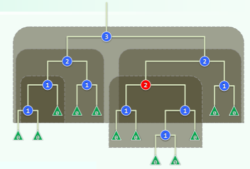

左式堆的左倾性

左式堆处处左倾：

对任何节点 x，都有 $n pl (l c (x)) \geq n pl (rc (x))$
由左倾性和 npl 的定义，可以推论： $n pl (x) = 1 + n pl (rc (x))$ ，即左式堆中每个节点的 npl 值仅与其右子有关
左倾性与堆序性，相容而不矛盾：
左式堆的子堆，必是左式堆
左式堆倾向于更多节点分布于左侧分支
- 这是否意味着，左子堆的规模和高度必然大于右子堆？——并不，请看上图的🔴红色节点

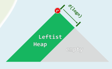
最右侧通路——右侧链

rChain (x)：从节点 x 出发，一直沿右分支前进直至空节点
尽管右孩子的高度可能大于左孩子，但由“每个节点的 npl 决定于右子”的推论可以得知， $n pl (x) = ∣ r C hain (x) ∣$ ——每个节点 npl 值等于其右侧链的长度。
特别地，rChain(r)的终点，即全堆中最浅的外部节点：
- $n pl (r) = ∣ r C hain (r) ∣ = d$
- 则该堆必然存在一棵以 r 为根、高度为 d 的满子树，下图的深绿色部分即是：
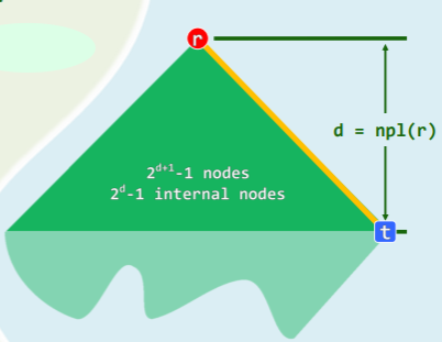
- 该满二叉树最少应包含 $2^{d + 1} - 1$ 个节点、 $2^{d} - 1$ 个内部节点，
- 同样，浅绿色的部分并非必然存在，因此上述节点数也是左式堆的节点数下限。
反之，包含 n 个节点的左式堆，右侧链长度必然不会长于 $d \leq ⌊ lo g_{2} (n + 1)⌋ - 1 = O (lo g n)$

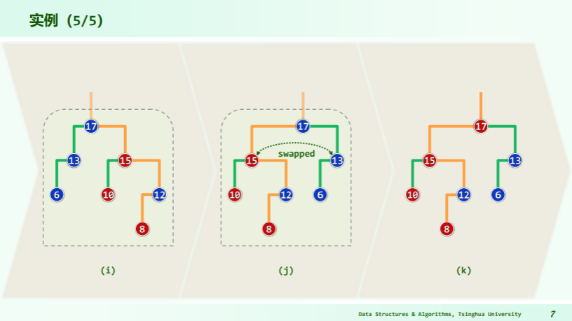
递归实现左式堆合并

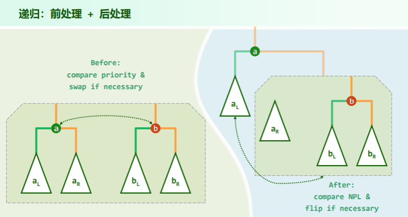
不妨设 a>=b，可以从右图看出——递归地将 a 的右子堆 $a_{R}$ 与 b 堆合并，然后作为节点 a 的右孩子替换原先的 $a_{R}$
为了保证左倾性，最后还需比较 a 的左右孩子的 npl 值——有必要时直接交换即可。

template <typename T> //合并以a和b为根节点的两个左式堆（递归版）
BinNodePosi<T> merge( BinNodePosi<T> a, BinNodePosi<T> b ) {
   if ( !a ) return b; //退化情况
   if ( !b ) return a; //退化情况
   if ( lt( a->data, b->data ) ) swap( a, b ); //确保a>=b
   ( a->rc = merge( a->rc, b ) )->parent = a; //将a的右子堆，与b合并
   if ( !a->lc || ( a->lc->npl < a->rc->npl ) ) //若有必要
      swap( a->lc, a->rc ); //交换a的左、右子堆，以确保右子堆的npl不大
   a->npl = a->rc ? a->rc->npl + 1 : 1; //更新a的npl
   return a; //返回合并后的堆顶
} //本算法只实现结构上的合并，堆的规模须由上层调用者负责更新

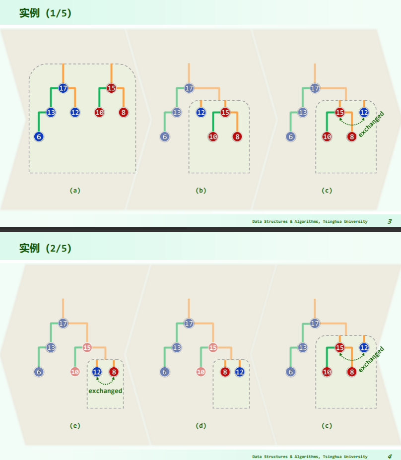
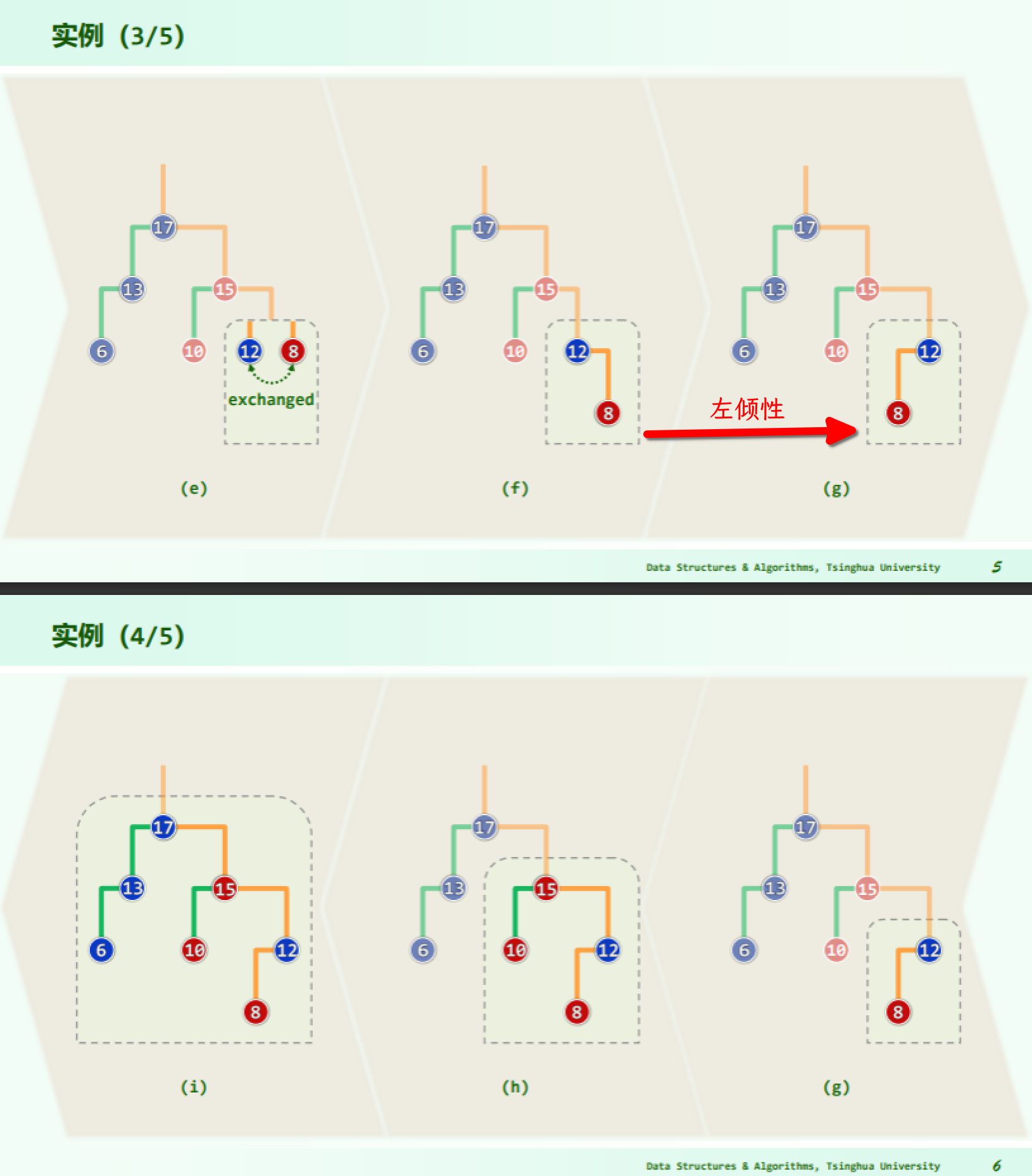
实例

左式堆合并的复杂度

递归版合并算法的所有递归实例，可以排成一个线性序列，因此实质上是线性递归，运行时间正比于递归深度。进一步地，递归只发生于两个待合并堆的最右侧通路上，因此若待合并堆的规模分别为 n 和 m，则其最右侧通路的长度不会超过 O (logn) 和 O (logm)，因此合并算法总体运行时间不超过 O (logn)+O (logm)=O (log (max (n, m)))

迭代实现合并

template <typename T> //合并以a和b为根节点的两个左式堆（迭代版）
BinNodePosi<T> merge( BinNodePosi<T> a, BinNodePosi<T> b ) {
   if ( !a ) return b; //退化情况
   if ( !b ) return a; //退化情况
   if ( lt( a->data, b->data ) ) swap( a, b ); //确保a>=b
   for ( ; a->rc; a = a->rc ) //沿右侧链做二路归并，直至堆a->rc先于b变空
      if ( lt( a->rc->data, b->data ) ) //只有在a->rc < b时才需做实质的操作
         { b->parent = a; swap( a->rc, b ); } //接入b的根节点（及其左子堆）
   ( a->rc = b )->parent = a; //直接接入b的残余部分（必然非空）
   for ( ; a; b = a, a = a->parent ) { //从a出发沿右侧链逐层回溯（b == a->rc）
      if ( !a->lc || ( a->lc->npl < a->rc->npl ) ) //若有必要
         swap( a->lc, a->rc ); //通过交换确保右子堆的npl不大
      a->npl = a->rc ? a->rc->npl + 1 : 1; //更新npl
   }
   return b; //返回合并后的堆顶
} //本算法只实现结构上的合并，堆的规模须由上层调用者负责更新

插入与删除

将 merge 作为左式堆的基本操作来实现 insert 和 delMax 操作：

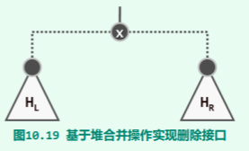
delMax：摘除 x 后，左右子堆进行一次 merge 即可：
insert：将 x 视作单个节点的堆，调用 merge 与之递归地合并即可：

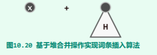
template <typename T> void PQ_LeftHeap<T>::insert( T e ) {
   _root = merge( _root, new BinNode<T>( e, NULL ) ); //将e封装为左式堆，与当前左式堆合并
   _size++; //更新规模
}

template <typename T> T PQ_LeftHeap<T>::delMax() {
   BinNodePosi<T> lHeap = _root->lc; if ( lHeap ) lHeap->parent = NULL; //左子堆
   BinNodePosi<T> rHeap = _root->rc; if ( rHeap ) rHeap->parent = NULL; //右子堆
   T e = _root->data; delete _root; _size--; //删除根节点
   _root = merge( lHeap, rHeap ); //合并原左、右子堆
   return e; //返回原根节点的数据项
}

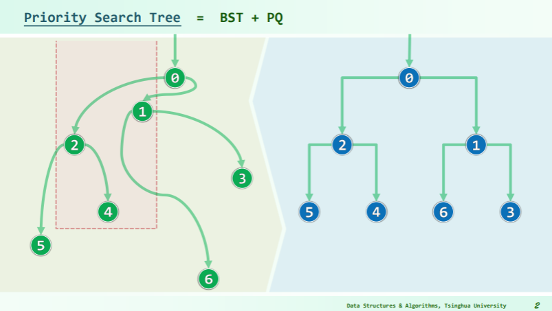
优先级搜索树

94-Priority-search-tree
In computer science, a priority search tree is a tree data structure for storing points in two dimensions. It was originally introduced by Edward M. McCreight.¹

It is effectively an extension of the priority queue with the purpose of improving the search time from O(n) to O(s + log n) time, where n is the number of points in the tree and s is the number of points returned by the search.

Description

The priority search tree is used to store a set of 2-dimensional points ordered by priority and by a key value. This is accomplished by creating a hybrid of a priority queue and a binary search tree.

The result is a tree where each node represents a point in the original dataset. The point contained by the node is the one with the lowest priority. In addition, each node also contains a key value used to divide the remaining points (usually the median of the keys, excluding the point of the node) into a left and right subtree. The points are divided by comparing their key values to the node key, delegating the ones with lower keys to the left subtree, and the ones strictly greater to the right subtree.²

结果是一个树，其中每个节点表示原始数据集中的一个点。节点包含的点是优先级最低的点。此外，每个节点还包含一个键值，用于将剩余点（通常是键的中位数，不包括节点的点）划分为左右子树。通过将它们的键值与节点键进行比较来划分点，将键较低的键委派给左侧子树，将严格较大的键委派给右侧子树。

Operations

Construction

The construction of the tree requires O(nlogn) time and O(n) space. A construction algorithm is proposed below:
tree construct_tree(data) {
  if length(data) > 1 {
  
    node_point = find_point_with_minimum_priority(data) // Select the point with the lowest priority
    
    reduced_data = remove_point_from_data(data, node_point)
    node_key = calculate_median(reduced_data) // calculate median, excluding the selected point
    
    // Divide the points 
    left_data = []
    right_data = []    
   
    for (point in reduced_data) {
      if point.key <= node_key
         left_data.append(point)
      else
         right_data.append(point)
    }

    left_subtree = construct_tree(left_data)
    right_subtree = construct_tree(right_data)

    return node // Node containing the node_key, node_point and the left and right subtrees

  } else if length(data) == 1 {
     return leaf node // Leaf node containing the single remaining data point
  } else if length(data) == 0 {
    return null // This node is empty
  }
}
Grounded range search

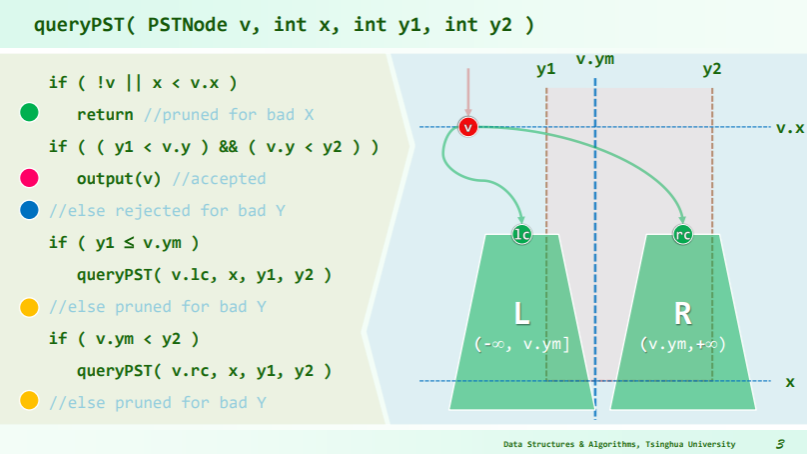
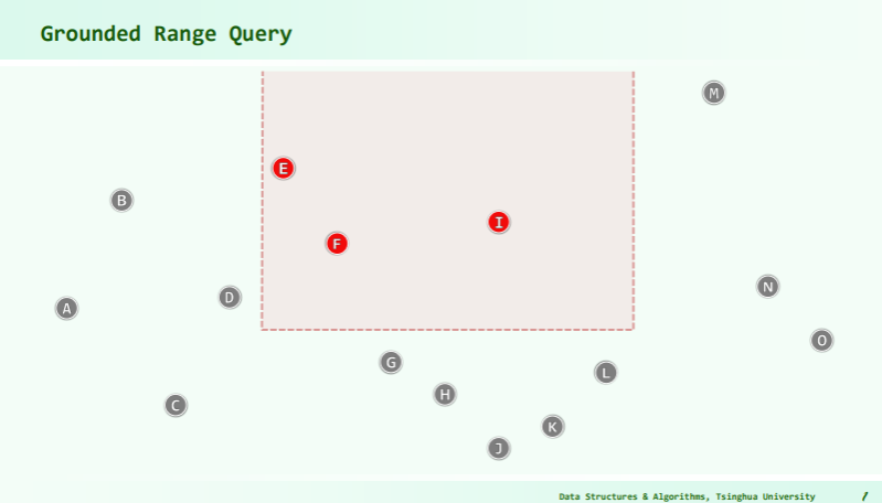
The priority search tree can be efficiently queried for a key in a closed interval and for a maximum priority value. That is, one can specify an interval [min_key, max_key] and another interval [-∞, max_priority] and return the points contained within it.

This is illustrated in the following pseudo code:
points search_tree(tree, min_key, max_key, max_priority) {
  root = get_root_node(tree) 
  result = []
  
  if get_child_count(root) > 0 {
      
    if get_point_priority(root) > max_priority
      return null // Nothing interesting will exist in this branch. Return

    if min_key <= get_point_key(root) <= max_key // is the root point one of interest?
       result.append(get_point(node))
   
    if min_key < get_node_key(root) // Should we search left subtree?
        result.append(search_tree(root.left_sub_tree, min_key, max_key, max_priority))

    if get_node_key(root) < max_key // Should we search right subtree?
        result.append(search_tree(root.right_sub_tree, min_key, max_key, max_priority))
      
    return result

  else { // This is a leaf node
    if get_point_priority(root) < max_priority and min_key <= get_point_key(root) <= max_key // is leaf point of interest?
       result.append(get_point(node))
  }
}
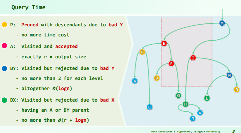
Quert time

Footnotes

McCreight, Edward (May 1985). “Priority search trees”. SIAM Journal on Scientific Computing. 14 (2): 257–276. doi: Priority Search Trees | SIAM Journal on Computing. ↩

Lee, D.T (2005). Handbook of Data Structures and Applications. London: Chapman & Hall/CRC. pp. 18–21. ISBN 1-58488-435-5. ↩

指向原始笔记的链接

🌰Senjl's Digital Garden🐉

Recent writing

Welcome to Senj's Digital Garden

4-地址空间

5-进程

探索

90-Priority_Queue

应用

ADT

实现