16-Stirling-Approximation

Intro

In mathematics, Stirling’s approximation (or Stirling’s formula) is an approximation for factorials. It is a good approximation, leading to accurate results even for small values of $n$ . It is named after James Stirling, though a related but less precise result was first stated by Abraham de Moivre.

One way of stating the approximation involves the logarithm of the factorial: $ln (n!) = n ln n - n + O (ln n),$ where the big O notation means that, for all sufficiently large values of $n$ , the difference between $ln (n!)$ and $n ln n - n$ will be at most proportional (正比于) to the logarithm.

In computer science applications such as the worst-case lower bound for comparison-based sorting, it is convenient to instead use the binary logarithm, giving the equivalent form
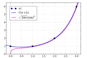
$lo g_{2} (n!) = n lo g_{2} n - n lo g_{2} e + O (lo g_{2} n) .$ The error term in either base can be expressed more precisely as $\frac{1}{2} lo g (2 πn) + O (\frac{1}{n})$ , corresponding to an approximate formula for the factorial itself, $n! \sim 2 πn (\frac{n}{e})^{n} .$ Here the sign $\sim$ means that the two quantities are asymptotic, that is, that their ratio tends to 1 as $n$ tends to infinity.

The following version of the bound holds for all $n \geq 1$ , rather than only asymptotically: $2 πn (\frac{n}{e})^{n} e^{\frac{1}{12 n + 1}} < n! < 2 πn (\frac{n}{e})^{n} e^{\frac{1}{12 n}} .$

Derivation

Roughly speaking, the simplest version of Stirling’s formula can be quickly obtained by approximating the sum $ln (n!) = j = 1 \sum n ln j$ with an integral: $j = 1 \sum n ln j \approx \int_{1}^{n} ln x d x = n ln n - n + 1.$

The full formula, together with precise estimates of its error, can be derived as follows. Instead of approximating $n!$ , one considers its natural logarithm, as this is a slowly varying function:

$ln (n!) = ln 1 + ln 2 + \dots + ln n .$

The right-hand side of this equation minus

$\frac{1}{2} (ln 1 + ln n) = \frac{1}{2} ln n$ is the approximation by the trapezoid rule of the integral $ln (n!) - \frac{1}{2} ln n \approx \int_{1}^{n} ln x d x = n ln n - n + 1,$

and the error in this approximation is given by the Euler–Maclaurin formula:

${\begin{aligned}\ln(n!)-{\tfrac {1}{2}}\ln n&={\tfrac {1}{2}}\ln 1+\ln 2+\ln 3+\cdots +\ln(n-1)+{\tfrac {1}{2}}\ln n\&=n\ln n-n+1+\sum {k=2}^{m}{\frac {(-1)^{k}B{k}}{k(k-1)}}\left({\frac {1}{n^{k-1}}}-1\right)+R_{m,n},\end{aligned}}$

where $B_{k}$ is a Bernoulli number, and R__m,n is the remainder term in the Euler–Maclaurin formula. Take limits to find that

$\lim _{n\to \infty }\left(\ln(n!)-n\ln n+n-{\tfrac {1}{2}}\ln n\right)=1-\sum {k=2}^{m}{\frac {(-1)^{k}B{k}}{k(k-1)}}+\lim {n\to \infty }R{m,n}.$

Denote this limit as $y$ . Because the remainder R__m,n in the Euler–Maclaurin formula satisfies

$R_{m,n}=\lim {n\to \infty }R{m,n}+O\left({\frac {1}{n^{m}}}\right),$

where big-O notation is used, combining the equations above yields the approximation formula in its logarithmic form:

$\ln(n!)=n\ln \left({\frac {n}{e}}\right)+{\tfrac {1}{2}}\ln n+y+\sum {k=2}^{m}{\frac {(-1)^{k}B{k}}{k(k-1)n^{k-1}}}+O\left({\frac {1}{n^{m}}}\right).$

Taking the exponential of both sides and choosing any positive integer $m$ , one obtains a formula involving an unknown quantity $e^{y}$ . For m = 1, the formula is

$n!=e^{y}{\sqrt {n}}\left({\frac {n}{e}}\right)^{n}\left(1+O\left({\frac {1}{n}}\right)\right).$

The quantity $e^{y}$ can be found by taking the limit on both sides as $n$ tends to infinity and using Wallis’ product, which shows that $e^{y}={\sqrt {2\pi }}$ . Therefore, one obtains Stirling’s formula: $n! = 2 πn (\frac{n}{e})^{n} (1 + O (\frac{1}{n}))$

Alternative derivations

An alternative formula for $n!$ using the gamma function is

$n!=\int _{0}^{\infty }x^{n}e^{-x},{\rm {d}}x.$ (as can be seen by repeated integration by parts). Rewriting and changing variables x = ny, one obtains $n!=\int _{0}^{\infty }e^{n\ln x-x},{\rm {d}}x=e^{n\ln n}n\int _{0}^{\infty }e^{n(\ln y-y)},{\rm {d}}y.$ Applying Laplace’s method one has $\int _{0}^{\infty }e^{n(\ln y-y)},{\rm {d}}y\sim {\sqrt {\frac {2\pi }{n}}}e^{-n},$ which recovers Stirling’s formula: $n!\sim e^{n\ln n}n{\sqrt {\frac {2\pi }{n}}}e^{-n}={\sqrt {2\pi n}}\left({\frac {n}{e}}\right)^{n}.$

Higher orders

In fact, further corrections can also be obtained using Laplace’s method. From previous result, we know that $\Gamma (x)\sim x^{x}e^{-x}$ , so we “peel off” this dominant term, then perform a change of variables, to obtain:

$x^{-x}e^{x}\Gamma (x)=\int _{\mathbb {R} }e^{x(1+t-e^{t})}dt$ Now the function $t\mapsto 1+t-e^{t}$ is unimodal, with maximum value zero. Locally around zero, it looks like $-t^{2}/2$ , which is why we are able to perform Laplace’s method. In order to extend Laplace’s method to higher orders, we perform another change of variables by $1+t-e^{t}=-\tau ^{2}/2$ . This equation cannot be solved in closed form, but it can be solved by serial expansion, which gives us $t=\tau -\tau ^{2}/6+\tau ^{3}/36+a_{4}\tau ^{4}+O(\tau ^{5})$ . Now plug back to the equation to obtain $x^{-x}e^{x}\Gamma (x)=\int {\mathbb {R} }e^{-x\tau ^{2}/2}(1-\tau /3+\tau ^{2}/12+4a{4}\tau ^{3}+O(\tau ^{4}))d\tau ={\sqrt {2\pi }}(x^{-1/2}+x^{-3/2}/12)+O(x^{-5/2})$ notice how we don’t need to actually find $a_4$ , since it is cancelled out by the integral. Higher orders can be achieved by computing more terms in $t=\tau +\cdots$ .

Thus we get Stirling’s formula to two orders:

$n!={\sqrt {2\pi n}}\left({\frac {n}{e}}\right)^{n}\left(1+{\frac {1}{12n}}+O\left({\frac {1}{n^{2}}}\right)\right).$

Complex-analytic version

A complex-analysis version of this method is to consider ${\frac {1}{n!}}$ as a Taylor coefficient of the exponential function $e^{z}=\sum _{n=0}^{\infty }{\frac {z^{n}}{n!}}$ , computed by Cauchy’s integral formula as

${\frac {1}{n!}}={\frac {1}{2\pi i}}\oint \limits _{|z|=r}{\frac {e^{z}}{z^{n+1}}},\mathrm {d} z.$

This line integral can then be approximated using the saddle-point method with an appropriate choice of contour radius $r=r_{n}$ . The dominant portion of the integral near the saddle point is then approximated by a real integral and Laplace’s method, while the remaining portion of the integral can be bounded above to give an error term.

Speed of convergence and error estimates

The relative error in a truncated Stirling series vs. $n$ , for 0 to 5 terms. The kinks in the curves represent points where the truncated series coincides with Γ(n + 1).

Stirling’s formula is in fact the first approximation to the following series (now called the Stirling series):

$n!\sim {\sqrt {2\pi n}}\left({\frac {n}{e}}\right)^{n}\left(1+{\frac {1}{12n}}+{\frac {1}{288n^{2}}}-{\frac {139}{51840n^{3}}}-{\frac {571}{2488320n^{4}}}+\cdots \right).$

An explicit formula for the coefficients in this series was given by G. Nemes. Further terms are listed in the On-Line Encyclopedia of Integer Sequences as A001163 and A001164. The first graph in this section shows the relative error vs. $n$ , for 1 through all 5 terms listed above. (Bender and Orszag p. 218) gives the asymptotic formula for the coefficients:

$A_{2j+1}\sim (-1)^{j}2(2j)!/(2\pi )^{2(j+1)}$ which shows that it grows superexponentially, and that by ratio test the radius of convergence is zero.

The relative error in a truncated Stirling series vs. the number of terms used

As n → ∞, the error in the truncated series is asymptotically equal to the first omitted term. This is an example of an asymptotic expansion. It is not a convergent series; for any particular value of $n$ there are only so many terms of the series that improve accuracy, after which accuracy worsens. This is shown in the next graph, which shows the relative error versus the number of terms in the series, for larger numbers of terms. More precisely, let S(n, t) be the Stirling series to $t$ terms evaluated at $n$ . The graphs show

$\left|\ln \left({\frac {S(n,t)}{n!}}\right)\right|,$ which, when small, is essentially the relative error.

Writing Stirling’s series in the form

$\ln(n!)\sim n\ln n-n+{\tfrac {1}{2}}\ln(2\pi n)+{\frac {1}{12n}}-{\frac {1}{360n^{3}}}+{\frac {1}{1260n^{5}}}-{\frac {1}{1680n^{7}}}+\cdots ,$ it is known that the error in truncating the series is always of the opposite sign and at most the same magnitude as the first omitted term.

More precise bounds, due to Robbins, valid for all positive integers $n$ are

${\sqrt {2\pi n}}\left({\frac {n}{e}}\right)^{n}e^{\frac {1}{12n+1}}<n!<{\sqrt {2\pi n}}\left({\frac {n}{e}}\right)^{n}e^{\frac {1}{12n}}.$ A looser version of this bound is that ![{\displaystyle {\frac {n! e^{n}}{n^{n+{\frac {1}{2}}}}}\in ({\sqrt {2\pi }}, e]}]( https://wikimedia.org/api/rest_v1/media/math/render/svg/809b4def5f2cd3a4f66ee3651b61f8c5d1f7e5b8 ) for all $n\geq 1$ .

Stirling’s formula for the gamma function

For all positive integers,

$n!=\Gamma (n+1),$ where Γ denotes the gamma function.

However, the gamma function, unlike the factorial, is more broadly defined for all complex numbers other than non-positive integers; nevertheless, Stirling’s formula may still be applied. If Re (z) > 0, then

$\ln \Gamma (z)=z\ln z-z+{\tfrac {1}{2}}\ln {\frac {2\pi }{z}}+\int _{0}^{\infty }{\frac {2\arctan \left({\frac {t}{z}}\right)}{e^{2\pi t}-1}},{\rm {d}}t.$

Repeated integration by parts gives

$\ln \Gamma (z)\sim z\ln z-z+{\tfrac {1}{2}}\ln {\frac {2\pi }{z}}+\sum {n=1}^{N-1}{\frac {B{2n}}{2n(2n-1)z^{2n-1}}},$

where $B_{n}$ is the $n$ th Bernoulli number (note that the limit of the sum as $N\to \infty$ is not convergent, so this formula is just an asymptotic expansion). The formula is valid for $z$ large enough in absolute value, when |arg (z)| < π − ε, where ε is positive, with an error term of O(z−2_N_+ 1). The corresponding approximation may now be written:

$\Gamma (z)={\sqrt {\frac {2\pi }{z}}},{\left({\frac {z}{e}}\right)}^{z}\left(1+O\left({\frac {1}{z}}\right)\right).$

where the expansion is identical to that of Stirling’s series above for $n!$ , except that $n$ is replaced with z − 1.

A further application of this asymptotic expansion is for complex argument z with constant Re (z). See for example the Stirling formula applied in Im (z) = t of the Riemann–Siegel theta function on the straight line .

Error bounds

For any positive integer $N$ , the following notation is introduced:

$\ln \Gamma (z)=z\ln z-z+{\tfrac {1}{2}}\ln {\frac {2\pi }{z}}+\sum \limits {n=1}^{N-1}{\frac {B{2n}}{2n\left({2n-1}\right)z^{2n-1}}}+R_{N}(z)$ and $\Gamma (z)={\sqrt {\frac {2\pi }{z}}}\left({\frac {z}{e}}\right)^{z}\left({\sum \limits {n=0}^{N-1}{\frac {a{n}}{z^{n}}}+{\widetilde {R}}_{N}(z)}\right).$

Then

$∣ R_{N} (z) ∣ R_{N} (z) \leq \frac{∣ B _{2 N} ∣}{2 N ( 2 N - 1 ) ∣ z ∣ ^{2 N - 1}} \times ⎩ ⎨ ⎧ 1 ∣ csc (ar g z) ∣ sec^{2 N} (\frac{a r g z}{2}) if ∣ ar g z ∣ \leq \frac{π}{4}, if \frac{π}{4} < ∣ ar g z ∣ < \frac{π}{2}, if ∣ ar g z ∣ < π, \leq (\frac{∣ a _{N} ∣}{∣ z ∣ ^{N}} + \frac{∣ a _{N + 1} ∣}{∣ z ∣ ^{N + 1}}) \times {1 ∣ csc (2 ar g z) ∣ if ∣ ar g z ∣ \leq \frac{π}{4}, if \frac{π}{4} < ∣ ar g z ∣ < \frac{π}{2} .$

For further information and other error bounds, see the cited papers.

A convergent version of Stirling’s formula

Thomas Bayes showed, in a letter to John Canton published by the Royal Society in 1763, that Stirling’s formula did not give a convergent series. Obtaining a convergent version of Stirling’s formula entails evaluating Binet’s formula:

$\int _{0}^{\infty }{\frac {2\arctan \left({\frac {t}{x}}\right)}{e^{2\pi t}-1}},{\rm {d}}t=\ln \Gamma (x)-x\ln x+x-{\tfrac {1}{2}}\ln {\frac {2\pi }{x}}.$

One way to do this is by means of a convergent series of inverted rising factorials. If

$z^{\bar {n}}=z(z+1)\cdots (z+n-1),$ then $\int _{0}^{\infty }{\frac {2\arctan \left({\frac {t}{x}}\right)}{e^{2\pi t}-1}},{\rm {d}}t=\sum {n=1}^{\infty }{\frac {c{n}}{(x+1)^{\bar {n}}}},$ where $c_{n}={\frac {1}{n}}\int _{0}^{1}x^{\bar {n}}\left(x-{\tfrac {1}{2}}\right),{\rm {d}}x={\frac {1}{2n}}\sum _{k=1}^{n}{\frac {k|s(n,k)|}{(k+1)(k+2)}},$ where s(n, k) denotes the Stirling numbers of the first kind. From this one obtains a version of Stirling’s series ${\begin{aligned}\ln \Gamma (x)&=x\ln x-x+{\tfrac {1}{2}}\ln {\frac {2\pi }{x}}+{\frac {1}{12(x+1)}}+{\frac {1}{12(x+1)(x+2)}}+\&\quad +{\frac {59}{360(x+1)(x+2)(x+3)}}+{\frac {29}{60(x+1)(x+2)(x+3)(x+4)}}+\cdots ,\end{aligned}}$ which converges when Re (x) > 0. Stirling’s formula may also be given in convergent form as $\Gamma (x)={\sqrt {2\pi }}x^{x-{\frac {1}{2}}}e^{-x+\mu (x)}$ where $\mu \left(x\right)=\sum _{n=0}^{\infty }\left(\left(x+n+{\frac {1}{2}}\right)\ln \left(1+{\frac {1}{x+n}}\right)-1\right).$

Versions suitable for calculators

The approximation

$\Gamma (z)\approx {\sqrt {\frac {2\pi }{z}}}\left({\frac {z}{e}}{\sqrt {z\sinh {\frac {1}{z}}+{\frac {1}{810z^{6}}}}}\right)^{z}$ and its equivalent form $2\ln \Gamma (z)\approx \ln(2\pi )-\ln z+z\left(2\ln z+\ln \left(z\sinh {\frac {1}{z}}+{\frac {1}{810z^{6}}}\right)-2\right)$ can be obtained by rearranging Stirling’s extended formula and observing a coincidence between the resultant power series and the Taylor series expansion of the hyperbolic sine function. This approximation is good to more than 8 decimal digits for z with a real part greater than 8. Robert H. Windschitl suggested it in 2002 for computing the gamma function with fair accuracy on calculators with limited program or register memory.

Gergő Nemes proposed in 2007 an approximation which gives the same number of exact digits as the Windschitl approximation but is much simpler:

$\Gamma (z)\approx {\sqrt {\frac {2\pi }{z}}}\left({\frac {1}{e}}\left(z+{\frac {1}{12z-{\frac {1}{10z}}}}\right)\right)^{z},$ or equivalently, $\ln \Gamma (z)\approx {\tfrac {1}{2}}\left(\ln(2\pi )-\ln z\right)+z\left(\ln \left(z+{\frac {1}{12z-{\frac {1}{10z}}}}\right)-1\right).$

An alternative approximation for the gamma function stated by Srinivasa Ramanujan (Ramanujan 1988[clarification needed]) is

$\Gamma (1+x)\approx {\sqrt {\pi }}\left({\frac {x}{e}}\right)^{x}\left(8x^{3}+4x^{2}+x+{\frac {1}{30}}\right)^{\frac {1}{6}}$ for x ≥ 0. The equivalent approximation for ln n! has an asymptotic error of 1/1400_n_3 and is given by $\ln n!\approx n\ln n-n+{\tfrac {1}{6}}\ln(8n^{3}+4n^{2}+n+{\tfrac {1}{30}})+{\tfrac {1}{2}}\ln \pi .$

The approximation may be made precise by giving paired upper and lower bounds; one such inequality is

${\sqrt {\pi }}\left({\frac {x}{e}}\right)^{x}\left(8x^{3}+4x^{2}+x+{\frac {1}{100}}\right)^{1/6}<\Gamma (1+x)<{\sqrt {\pi }}\left({\frac {x}{e}}\right)^{x}\left(8x^{3}+4x^{2}+x+{\frac {1}{30}}\right)^{1/6}.$

History

The formula was first discovered by Abraham de Moivre in the form

$n! \sim [constant] \cdot n^{n + \frac{1}{2}} e^{- n} .$

De Moivre gave an approximate rational-number expression for the natural logarithm of the constant. Stirling’s contribution consisted of showing that the constant is precisely ${\sqrt {2\pi }}$ .

References

^
^ Jump up to: a b Le Cam, L. (1986), “The central limit theorem around 1935”, Statistical Science, 1 (1): 78–96, doi: 10.1214/ss/1177013818, JSTOR 2245503, MR 0833276; see p. 81, “The result, obtained using a formula originally proved by de Moivre but now called Stirling’s formula, occurs in his ‘Doctrine of Chances’ of 1733.”
^ Jump up to: a b Pearson, Karl (1924), “Historical note on the origin of the normal curve of errors”, Biometrika, 16 (3/4): 402–404 [p. 403], doi: 10.2307/2331714, JSTOR 2331714, I consider that the fact that Stirling showed that De Moivre’s arithmetical constant was ${\sqrt {2\pi }}$ does not entitle him to claim the theorem, […]
^ Flajolet, Philippe; Sedgewick, Robert (2009), Analytic Combinatorics, Cambridge, UK: Cambridge University Press, p. 555, doi: 10.1017/CBO9780511801655, ISBN 978-0-521-89806-5, MR 2483235, S2CID 27509971
^ Olver, F. W. J.; Olde Daalhuis, A. B.; Lozier, D. W.; Schneider, B. I.; Boisvert, R. F.; Clark, C. W.; Miller, B. R. & Saunders, B. V., “5.11 Gamma function properties: Asymptotic Expansions”, NIST Digital Library of Mathematical Functions, Release 1.0.13 of 2016-09-16
^ Nemes, Gergő (2010), “On the coefficients of the asymptotic expansion of $n!$ ”, Journal of Integer Sequences, 13 (6): 5
^ Bender, Carl M.; Orszag, Steven A. (2009). Advanced mathematical methods for scientists and engineers. 1: Asymptotic methods and perturbation theory (Nachdr. ed.). New York, NY: Springer. ISBN 978-0-387-98931-0.
^ Robbins, Herbert (1955), “A Remark on Stirling’s Formula”, The American Mathematical Monthly, 62 (1): 26–29, doi: 10.2307/2308012, JSTOR 2308012
^ Spiegel, M. R. (1999), Mathematical handbook of formulas and tables, McGraw-Hill, p. 148
^ Schäfke, F. W.; Sattler, A. (1990), “Restgliedabschätzungen für die Stirlingsche Reihe”, Note di Matematica, 10 (suppl. 2): 453–470, MR 1221957
^ G. Nemes, Error bounds and exponential improvements for the asymptotic expansions of the gamma function and its reciprocal, Proc. Roy. Soc. Edinburgh Sect. A 145 (2015), 571–596.
^ Bayes, Thomas (24 November 1763), “A letter from the late Reverend Mr. Thomas Bayes, F. R. S. to John Canton, M. A. and F. R. S.” (PDF), Philosophical Transactions of the Royal Society of London Series I, 53: 269, Bibcode: 1763RSPT… 53.. 269B, archived (PDF) from the original on 2012-01-28, retrieved 2012-03-01
^ Artin, Emil (2015). The Gamma Function. Dover. p. 24.
^ Toth, V. T. Programmable Calculators: Calculators and the Gamma Function (2006) Archived 2005-12-31 at the Wayback Machine.
^ Nemes, Gergő (2010), “New asymptotic expansion for the Gamma function”, Archiv der Mathematik, 95 (2): 161–169, doi: 10.1007/s00013-010-0146-9, S2CID 121820640
^ Karatsuba, Ekatherina A. (2001), “On the asymptotic representation of the Euler gamma function by Ramanujan”, Journal of Computational and Applied Mathematics, 135 (2): 225–240, Bibcode: 2001JCoAM. 135.. 225K, doi: 10.1016/S0377-0427 (00) 00586-0, MR 1850542
^ Mortici, Cristinel (2011), “Ramanujan’s estimate for the gamma function via monotonicity arguments”, Ramanujan J., 25 (2): 149–154, doi: 10.1007/s11139-010-9265-y, S2CID 119530041
^ Mortici, Cristinel (2011), “Improved asymptotic formulas for the gamma function”, Comput. Math. Appl., 61 (11): 3364–3369, doi: 10.1016/j.camwa. 2011.04.036.
^ Mortici, Cristinel (2011), “On Ramanujan’s large argument formula for the gamma function”, Ramanujan J., 26 (2): 185–192, doi: 10.1007/s11139-010-9281-y, S2CID 120371952.

🌰Senjl's Digital Garden🐉

Recent writing

Welcome to Senj's Digital Garden

4-地址空间

5-进程

探索

References

1. ^
2. ^ Jump up to: a b Le Cam, L. (1986), ā€œThe central limit theorem around 1935ā€, Statistical Science, 1 (1): 78ā€“96, doi: 10.1214/ss/1177013818, JSTORĀ 2245503, MRĀ 0833276; see p. 81, ā€œThe result, obtained using a formula originally proved by de Moivre but now called Stirlingā€™s formula, occurs in his ā€˜Doctrine of Chancesā€™ of 1733.ā€
3. ^ Jump up to: a b Pearson, Karl (1924), ā€œHistorical note on the origin of the normal curve of errorsā€, Biometrika, 16 (3/4): 402ā€“404 [p. 403], doi: 10.2307/2331714, JSTORĀ 2331714, I consider that the fact that Stirling showed that De Moivreā€™s arithmetical constant was {\sqrt {2\pi }} does not entitle him to claim the theorem, [ā€¦]